Authors:
(1) Omer Rathore, Department of Physics, Durham University;
(2) Alastair Basden, Department of Physics, Durham University;
(3) Nicholas Chancellor, Department of Physics, Durham University and School of Computing, Newcastle University;
(4) Halim Kusumaatmaja, Department of Physics, Durham University and Institute for Multiscale Thermofluids, School of Engineering, The University of Edinburgh.
Table of Links
Methods
Results
Conclusions and Outlook, Acknowledgements, and References
Grid Based Application
In the following discussion, the concept of “imbalance” will serve as an important metric, and is defined in Equation 9 for each processor in a given partition.

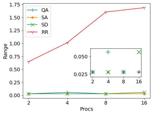
A more top-level performance metric to consider is the maximum disparity in processor load. This quantifies time spend by the faster processor waiting for the slowest one to complete its tasks before advancing to the next simulation time step. This range between the fastest and slowest processors is graphically represented for the the same configurations as before in Figure 5. The round robin strategy emerges as the least efficient, leading to considerable CPU time wastage. In such a protocol, processors with fewer tasks remain idle for prolonged periods of time while awaiting the completion of assignments by processors with heavier loads. On the other hand, QA typically provides more balanced solutions. However, a distinct “kink” is observed when partitioning across four processors. This kink indicates a drop in solution quality compared to the results achieved with Simulated Annealing (SA) and Steepest Descent (SD). This suboptimal performance can be attributed partially to the inherent stochastic nature of QA, where the optimal solution is not guaranteed in any specific run. However SA is also stochastic and performs better, so the QA solution may also be influenced by problem-specific parameters, a topic slated for in-depth evaluation in subsequent sections. Notably, when the computational work is distributed across a higher number of processors (e.g. 16), both QA and SA appear to surpass SD, which starts to falter due to the emergence of sub-optimal local minima in the increasingly fragmented energy landscape resulting from recursive partitioning. This suggests that, for some
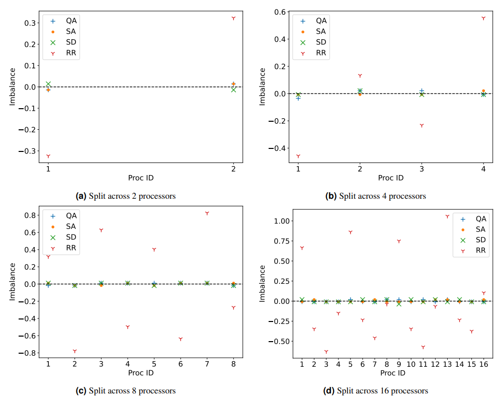
configurations, it may be possible to obtain an improvement even over more advanced classical methods such as SD.
The aforementioned results pertain to a fixed number of anneals and a single invocation of the D-Wave API. While D-Wave functions in the minorminer library[77], [78] effectively optimize the embedding of the logical problem onto the physical qubits, it is worthwhile noting that this algorithm is heuristic. A single call to the D-Wave API means that only one embedding configuration is utilized. Under ideal conditions, this alone should not significantly impact the results. However, for the ensuing statistical analysis, five distinct embedding configurations were pre-computed and stored in order to map the problem to different physical qubits. When studying the effect of a parameter, for example number of anneals, each configuration underwent five separate runs using the pre-computed embeddings prior to averaging. This aims to minimize potential biases in the hardware that might undesirably affect the outcomes.
So far only the lowest energy solution was considered from the range of possible configurations that arise from QA. Despite demonstrating good performance this begs the important question of how likely is this to actually be observed in practice. Due to the inherent nature of load balancing requiring repeated redistribution after some number of time steps, it is not necessarily a stringent requirement to have the best possible solution each time. In fact, it may suffice to have something close enough.
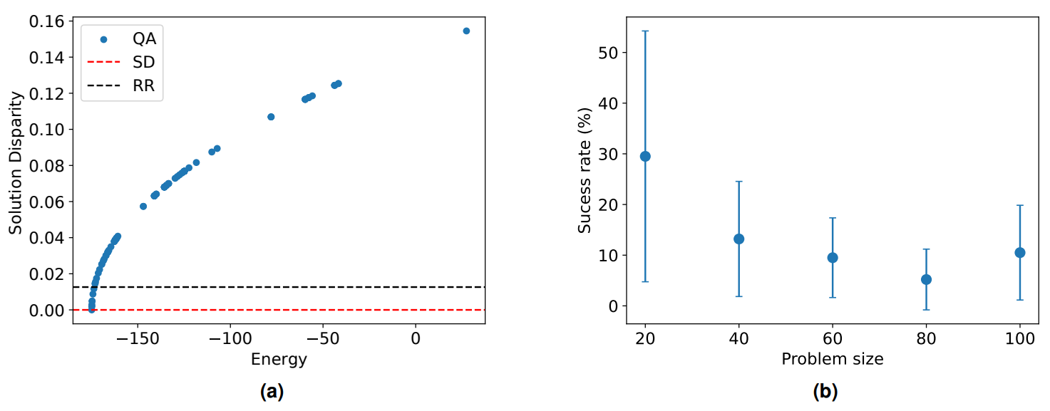
Figure 6a attempts to illustrate this by plotting all the samples from a single run with a hundred anneals for a small problem size of 50 grids during a single partition. The energy output from a QA is arbitrarily scalable, therefore the actual numerical value is of little consequence other than the trend of a lower energies representing better solutions. This is in accordance with
the corresponding solution disparity as defined in Equation 10,

The solution disparity is thus the difference between assigned work loads for a single partition normalised by the work resulting from a perfect split. In other words, a lower solution disaparity corresponds with better solution quality.
Included in Figure 6a for comparison are the solution disparities obtained from the deterministic round robin and steepest descent methods. Even with such a small number of anneals, the best (i.e. lowest energy) quantum solution has the same degree of imbalance as SD, with both methods arriving at the optimum solution for this configuration. There is also a significant proportion of the annealing samples that perform worse than SD but better than RR. These are the blue markers in between the two dotted, horizontal lines and suggest some degree of resilience in the method despite being heuristic. The spread of points with a higher disparity than the black dotted line are clearly inferior and hold little value.
Figure 6b illustrates the variation in the percentage of QA solutions that represent an improvement over RR across different problem sizes, based on results from 100 anneals. It is evident that the frequency of sub-optimal solutions escalates with the increase in problem size, indicating a relative under-performance compared to simulated annealing, which achieves a success rate of approximately 90% across this range of problem sizes. Despite this, the quality of the most optimal solution obtained from both QA and SA remains the same.
This observation suggests that while QA has the potential to match the performance of more sophisticated classical algorithms, it does so for a limited fraction of the generated solutions. Given that QA is inherently a probabilistic method, it naturally involves generating a large number of samples to increase the likelihood of obtaining a high-quality solution. The advantage of QA lies in its ability to rapidly produce samples, with each annealing process taking just microseconds. As a result, even a relatively low success rate can, in practice, almost guarantee the identification of at least one successful outcome, which is often the primary goal. This efficiency in sample generation underscores the practical viability of QA. Furthermore, it should be noted that at this point no a priori optimisation for QA of user defined parameters such as number of anneals and chain strength have been provided to the annealer. Consequently, not only is the number of anneals very small here, but there is also a considerable number of chain breaks for problem sizes of 40 and more which can significantly degrade performance.
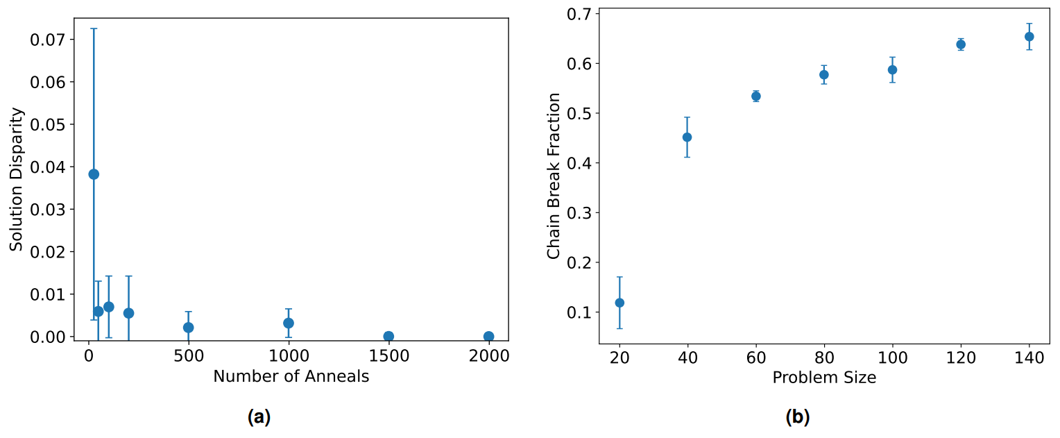
In order to evaluate the impact of parameter choices, the more challenging case with 100 grids is partitioned while changing the number of anneals. Figure 7a illustrates how the solution quality varies with anneals for a fixed problem size. Each configuration was repeated five times with a pre-computed embedding and the average lowest energy solution is shown here with error bars reflecting its standard deviation. As expected, increasing the number of anneals increases the likelihood of finding a near optimum solution. Although the mean quality seems to plateau relatively early in terms of magnitude, increasing anneals has significant impact on reducing error margins and thus the reliability of obtaining said solution. Considering the relatively small number of anneals needed to drastically improve solution quality as well as the cheap computation cost of each
anneal, it is evident that this is likely not a limiting factor.
Thus, the main roadblock to achieving scalability is unlikely to be the number of required anneals, but is perhaps the susceptibility to chain breaks. The Ising model here forms a fully connected graph while annealing hardware has limited physical couplings. This results in minor embedding forming chains of physical qubits to represent the same logical qubit. However it is evident in Figure 7b that the default chain strength, calculated using uniform torque compensation, quickly becomes inadequate at larger problem sizes. The significant increase in chain break fraction (CBF) as the number of patches/grids requiring partitioning increases result in a decision problem that is by default resolved via majority voting. At values as high as those seen in Figure 7b this has severe implications for the utility and robustness of the method for realistic applications where the number of patches/grids needing to be partitioned will be well over a hundred if not in the thousands or more.
One solution to this is overriding the default chain strength scheme and manually setting stronger chains. This approach was explored in Figure 8a for a fixed problem size involving a hundred grids. The chain strength in the graph is defined by the multiplier applied to the max value in the data set. In other words, a chain strength of 1000 here means a value a thousand times larger than the maximum number in the set. It is evident that the value required to maintain an acceptable fraction of breaks is several orders of magnitude higher than one might have anticipated from the size of numbers being partitioned. It is unclear if it would have been possible to predict this a priori and how this trend would scale at realistic problem sizes.
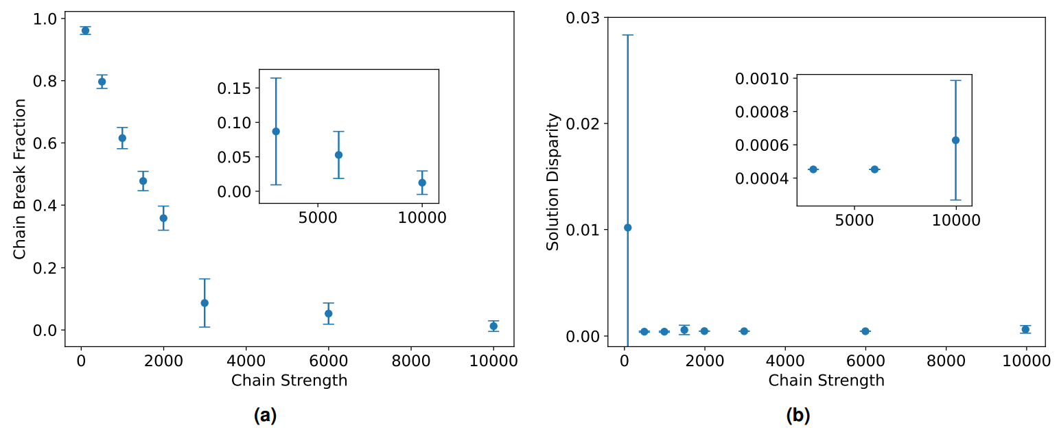
It is also well known that blindly increasing the chain strength is not the perfect solution. Having qubits in very rigid chains can make them inflexible and less efficient at exploring the solution space. It can also wash out the other energy scales so that they are less than the device temperature and therefore lead to effectively random solutions. Furthermore, the energy penalty from the chain term can start rivalling the energy contribution from the actual Ising model if it grows too large and this can introduce a bias in the solution. Thus there is a balancing act to be performed, where clearly the default scheme is not adequate for the problem being considered here, yet too strong a chain is also undesirable. This is demonstrated in Figure 8b where increasing the chain strength brings a large improvement in solution quality. However, with very strong chains the solution does begin to degrade again. The silver lining is that there seems to be a very large region of the state space that results in good solutions.
Taken together, the analysis here suggests that QA exhibits notable improvements when compared to basic classical algorithms like RR. Furthermore, QA demonstrates the capability to achieve solutions of comparable quality to those generated by more sophisticated algorithms, such as SA and SD. However, to attain such high-quality solutions consistently, QA may necessitate preliminary adjustments or tuning, highlighting the importance of optimizing the quantum annealing process for specific problem sets. It is important to acknowledge that the scope of problem sizes investigated in this study is constrained by the limitations of current quantum computing hardware. As hardware capabilities improve, it is anticipated that these limitations will decrease, thereby expanding the range of problem sizes that can be efficiently addressed. The complexity of the energy landscape in this section is also limited, whereby advanced classical methods are able to arrive at near optimum solutions without being excessively hindered by local minima traps. We anticipate QA will be more advantageous over classical approaches for more complex energy landscapes with deep local minima traps. This highlights a crucial aspect of quantum annealing: identifying and formulating problem sets that truly leverage the unique strengths of quantum algorithms to solve problems that are intractable for classical methods.
This paper is available on arxiv under CC BY 4.0 DEED license.
